The dictionary does all of its colour reasoning in OKLab — classifying shades, measuring ΔTartan, drawing dye-range maps. Those maps always show colours inside a gamut. This story asks the opposite question: where is the outer edge of all physically possible colour — the locus of pure monochromatic light, the curve that draws the famous horseshoe of the CIE 1931 chromaticity diagram — when you plot it in OKLab?
Why this is not a straight translation
The CIE 1931 horseshoe is a chromaticity diagram. It lives in a projective plane: the tristimulus values are normalised, \( x = X/(X+Y+Z),; y = Y/(X+Y+Z) \), so intensity is divided out and each monochromatic wavelength collapses to a single point.
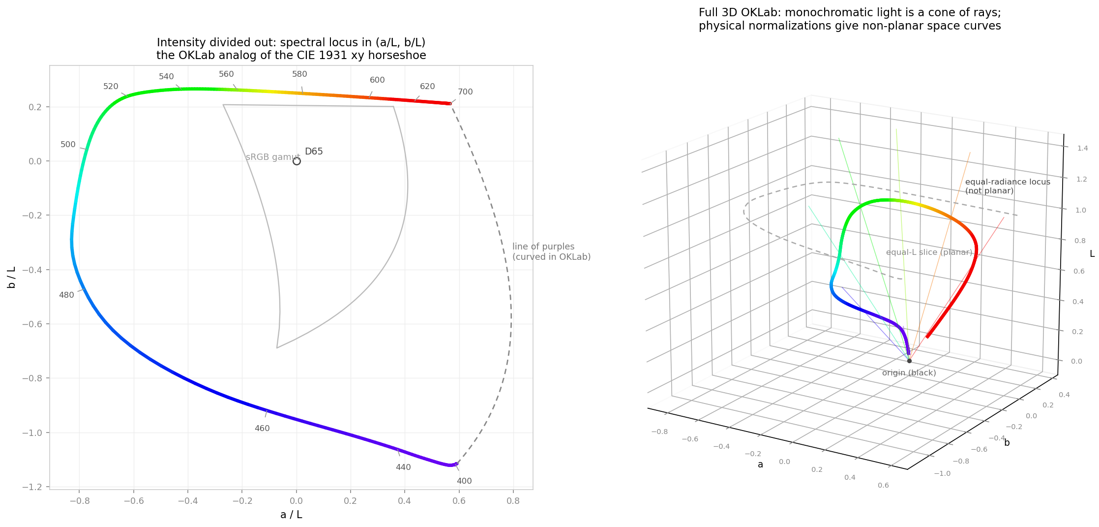
OKLab is a three-dimensional appearance space. A monochromatic light has a free intensity, so in OKLab it is not a point at all — it is a whole ray, and the set of all monochromatic lights is a cone of rays through the origin (right panel above). Before you can plot "the" locus you must choose how to cut that cone, and different cuts give genuinely different shapes — including ones that do not lie in any plane.
The rays are straight — a small derivation
OKLab is defined (Ottosson) as two matrix maps around a cube root, with no offsets:
$$ \mathrm{Lab} = M_2 \cdot \sqrt[3]{,M_1 \cdot \mathrm{XYZ},} $$
Scale the intensity of a light by \(k\): XYZ becomes \(k,\mathrm{XYZ}\), the LMS vector becomes \(k,\mathrm{LMS}\), the cube root turns that into a uniform factor \(k^{1/3}\), and the final linear map preserves it. So
$$ (L, a, b) ;\longmapsto; (k^{1/3}L,; k^{1/3}a,; k^{1/3}b). $$
Every intensity ray in XYZ maps to a straight ray through the OKLab origin. Two useful consequences fall straight out:
- OkLCH hue is intensity-invariant. \(h = \operatorname{atan2}(b, a)\) is unchanged by the common factor. A wavelength has a well-defined OKLab hue angle.
- The ratios \(a/L\) and \(b/L\) are intensity-invariant. They are the natural OKLab analog of the \((x, y)\) chromaticity coordinates.
Cut 1 — divide intensity out (the horseshoe's analog)
Plot \((a/L,; b/L)\) for each wavelength (left panel). The recipe:
- For each wavelength take the CIE 1931 2° colour-matching-function triple \((\bar{x}, \bar{y}, \bar{z})\) as the XYZ of that monochromatic light — the scale is irrelevant, that is the point.
- Convert XYZ → OKLab with a signed cube root: spectral stimuli sit far outside any
display gamut and can push one LMS component slightly negative. (
np.cbrtis signed;pow(x, 1/3)is not.) - Plot \((a/L, b/L)\). D65 lands exactly at the origin, because OKLab is normalised so that D65 white has \(a = b = 0\).
The result is recognisably the horseshoe's cousin: red through green along the top, the long blue sweep down the left, violet curling in at the bottom right, everything beyond ~650 nm piling up at the red corner just as it does in \(xy\). The sRGB gamut — the RGB cube's edges pushed through the same projection — floats inside it around the white point.
One familiar feature breaks: the line of purples is not straight. In \(xy\) it is straight because chromaticity is a projective-linear map, and mixtures of two lights lie on the segment between them. The cube root destroys that linearity, so in OKLab the purple boundary must be computed — mix the endpoint stimuli, \(t \cdot \mathrm{XYZ}(400,\text{nm}) + (1-t)\cdot \mathrm{XYZ}(700,\text{nm})\), and map each mixture. It comes out bowed (dashed curve).
Cut 2 — fix the physics (and leave the plane)
Dividing by \(L\) is a mathematician's cut. A physicist would instead fix a normalisation and keep all three coordinates:
- Equal radiance — plot the CMF triple directly. This is the solid 3D curve in the right panel: lightness peaks near 555 nm where the eye is most sensitive and dives toward the origin (black) at both spectral ends, where the eye barely responds at all.
- Equal luminance — scale every wavelength to the same \(Y\). Also a space curve, with the tails now flung far outward instead of collapsing.
Neither curve lies in any plane — the spectral locus in OKLab is intrinsically a three-dimensional object. Only the artificial constant-\(L\) slice of the cone (dashed ring) is planar, and that is the shape the left panel flattens.
Practical notes
- Use the real CMF table, not analytic fits. A first draft of the diagram used the
Wyman–Sloan–Shirley Gaussian approximation and the locus grew a false loop at the violet
end: the fitted \(\bar{y}\) tail is ~3× too large below 410 nm, and chromaticity is a
ratio of near-zero numbers there, so tail error dominates. The bundled
ciexyz31_1.csvis the CVRL 1 nm table; the full derivation is in the bundledoklab_locus_final.py. - OKLab is an extrapolation out there. It was fitted to display-gamut data, so near the spectral locus the space is a smooth extension, not a perceptual measurement. That is fine for plotting and for hue bookkeeping, but chroma distances near the edge should not be read as calibrated ΔE — a caveat that matters when we reason about how far a dye gamut could ever be pushed.
For the dictionary the takeaway is orientation: our dye-range maps live on constant-\(L\) slices, and this curve is the absolute boundary those slices can never cross — the rim of colour itself.